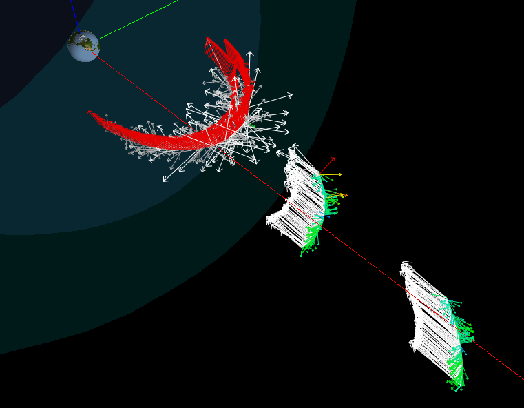Four THEMIS spacecraft displaying FGM (magnetic field as rainbow colored vectors) and ESA (electron velocity as grayscale vectors) products. A parametrically modeled bow shock and magnetopause are shown as blue, semi-transparent surfaces.

Several THEMIS spacecraft showing changes in magnetic field vectors at magnetospheric boundaries.

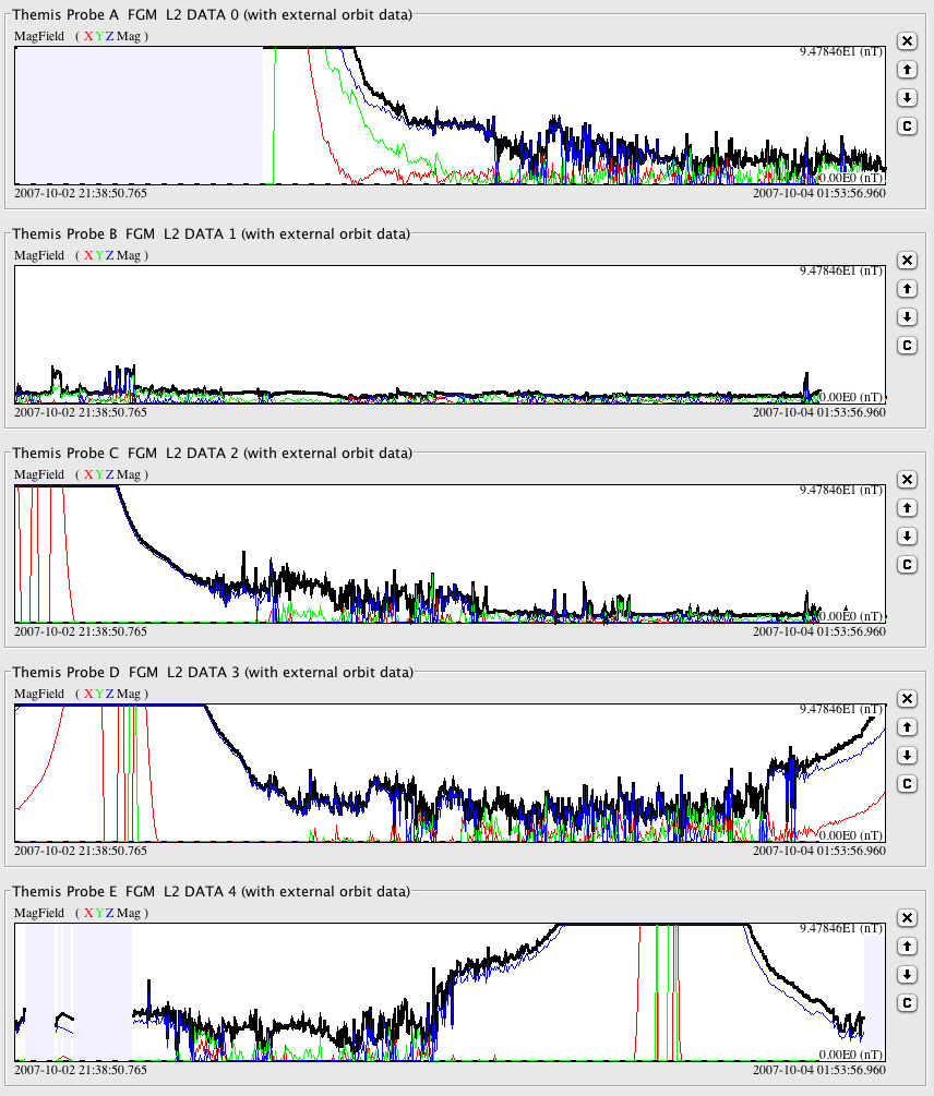Panel plot of the 3-D image above; 2-D and 3-D views can be shown simultaneously and synchronized in time.

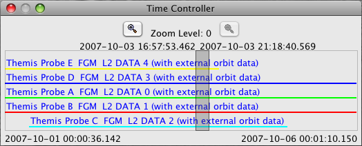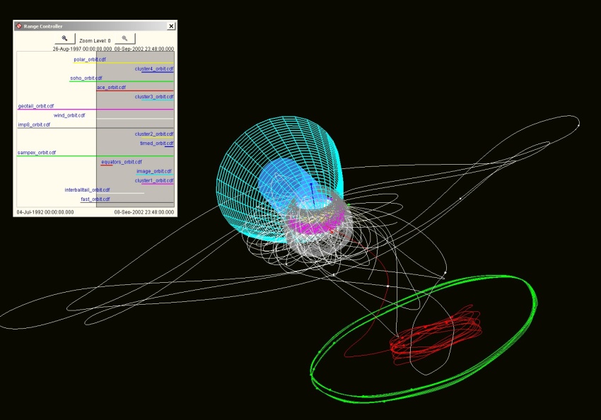
Interactive time slider showing currently-loaded spacecraft and selected range.

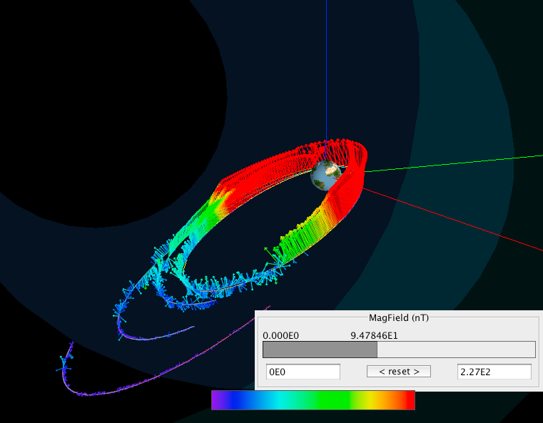
An overview of the orbits of 15 spacecraft over their entire mission lifetimes. Modeled bow shock and magnetopause surfaces and a properly rotating Earth with its magnetic pole provide the proper context. The user can examine both the extent of the spacecraft coverage and, by selecting a small time range for viewing, determine specific configurations of spacecraft useful for a given study. Furthermore, ViSBARD provides access to several data repositories so that the orbits and data can be retrieved from within the application.

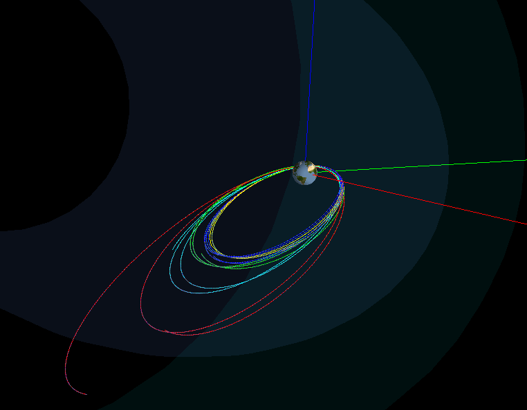
Five days of orbits for five THEMIS spacecraft.

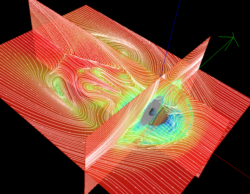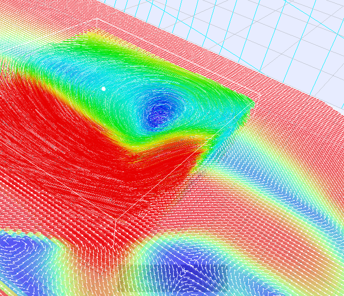
Axis-aligned cut planes of OpenGGCM MHD data. In this case, plasma flow velocity is double-encoded: its magnitude is represented by color and its path by streamlines.

In the general case, scalar and vector quantities can be arbitrarily mapped to colors, vectors, streamlines, and contour lines.

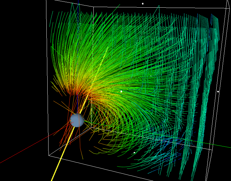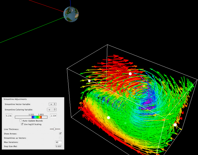
Magnetic field lines are traced in 3-D from a BATS-R-US MHD model run. Streamline variables, colors, seeding, and the region of interest can be adjusted interactively.

OpenGGCM flow data is shown with a Z=0 cut plane and a 3-D volume of streamlines.

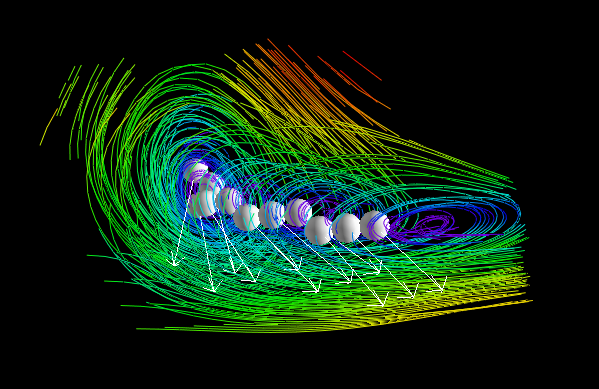
Flow vortex shown in OpenGGCM data.

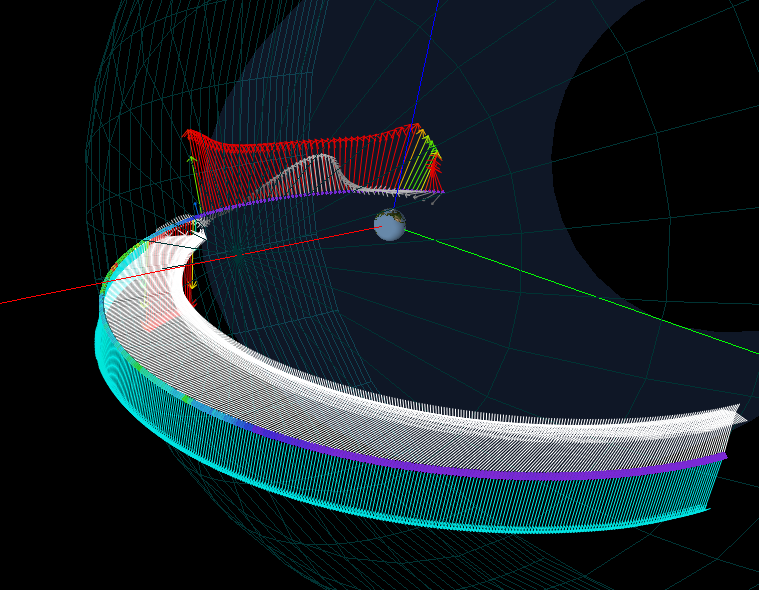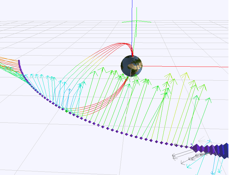
MHD data can also be interpolated along spacecraft orbits. In this case, magnetic field vectors (rainbow colored) and plasma flow (grayscale) data from a BATS-R-US model run is shown along a Geotail orbit.

This enables easy comparison between spacecraft observations and MHD model results as shown in this Geotail orbit: observed magnetic field data is shown as rainbow colored vectors and model results in grayscale.

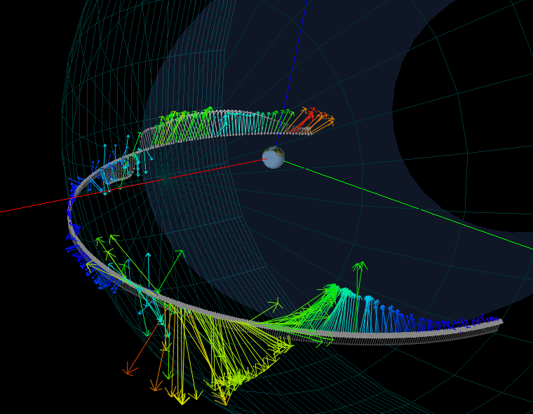
Feature detection algorithms can be applied to MHD data through ViSBARD's architecture. A vortex-finding algorithm clustered its results as shown; vortex centers are shown as spheres and its vorticity at that point as a vector.

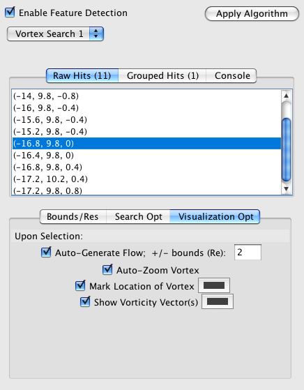
Vortex search GUI, showing its raw results. Once an individual result is selected, the application can perform specific visualization tasks on it.

Tsyganenko magnetic field line models (87, 89, 96, 2001) can be used to generate the last closed field lines. Source code courtesy of Orbit Visualization Toolkit (OVT) team.

Field lines can be generated to pass through a selected data point and its neighbors.

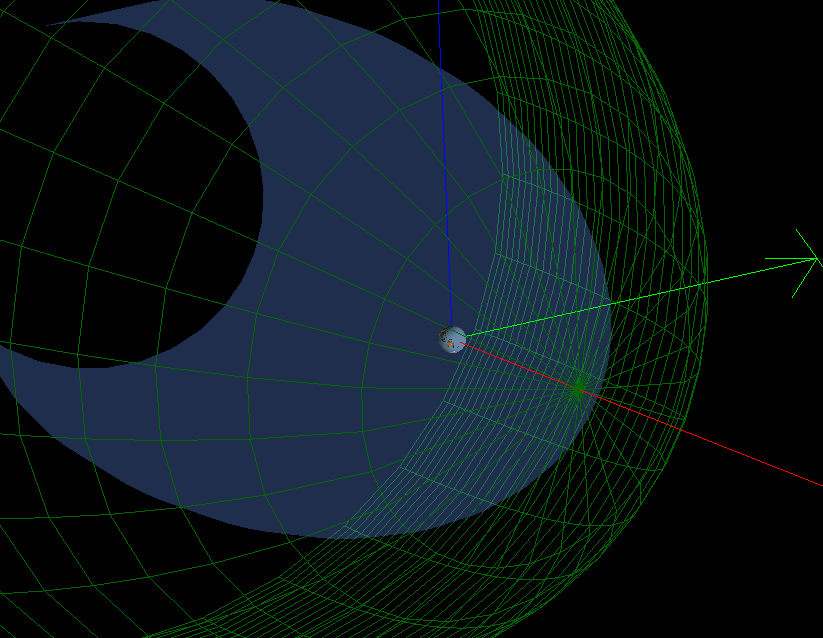Fairfield's bow shock surface (green mesh) and Sibeck's Magnetopause (blue semi-transparent surface) can also be dynamically adjusted based on OMNI data or entered manually.

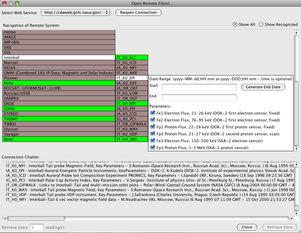
Remote data repositories can be browsed from within ViSBARD via their Java Web Services interface. Data can then be directly retrieved and imported into the application. Currently-supported repositories include CDAWeb, SSCWeb, and the VSPO.

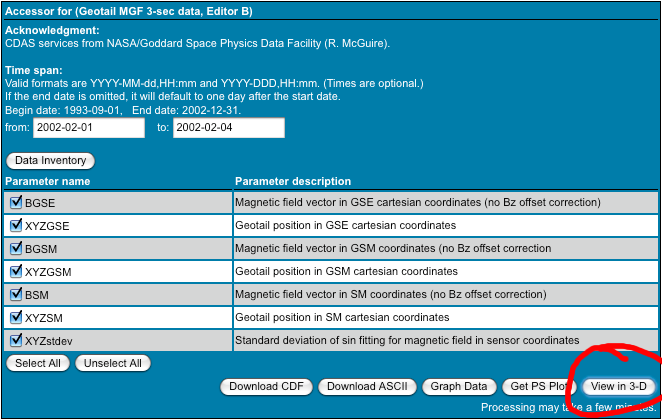
Data can be "pushed" to ViSBARD via the web interface of the Virtual Space Physics Observatory (VSPO) for supported data products. Just click the "View in 3-D" button if it exists.

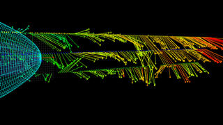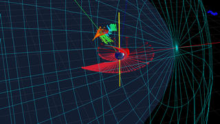
Three spacecraft ahead of the Earth's bow shock measure the magnetic field as it is carried by the solar wind towards the Earth. Their positions as projected according to the flow speed are noted with the small glyph (Wind = yellow, Geotail = blue, IMP-8 = green). The spacecraft actually move very little over the time interval shown, but a spatial picture emerges when we use a knowledge of the wind velocity to spread the vectors out according to how they flowed past the point of observation. Arrows on the satellite glyphs indicate the magnitude and direction of the magnetic field while the color also represents the intensity (red being the highest, blue the lowest).

As the wind flows, we can rapidly obtain information on the extended geometry of convected structures. The wire-frame at the left is a representation of the Earth's bow shock (about 100 Earth radii across in what is shown) that shows where the Sun's magnetic field would begin to be affected by that the Earth. (The effect of the interaction is not shown.)

Animator: Tom Bridgman / Scientific Visualization Studio

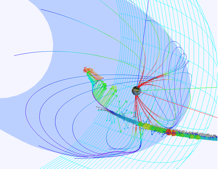
In this visualization created from ViSBARD screenshots, we see the magnetic field as measured from six different satellites. The position of each spacecraft is marked by a small color glyph (ACE = yellow, Cluster = dark blue, Geotail = green, GOES 10 = red, Polar = light blue, Wind = purple). The direction of the arrow signifies the direction of the magnetic field while the color represents the intensity (red being the highest, blue the lowest). The magnetic pole of the Earth is in yellow, and it rotates properly as the animation proceeds.

This view of the magnetic storm shows highly disturbed fields at geosynchronous orbit (GOES), many crossings of the 'magntotail current sheet' where the field changes sign and points at the opposite pole of the Earth, close encounters with the Earth (large red fields that are truncated to keep the arrows from becoming huge), and the entry from the back of the picture of Wind and Geotail through the bow shock (wire-frame) and magnetopause (sometimes visible as a transparent surface).

Data for this animation was taken from a solar storm on October 7, 2002.

Animator: Tom Bridgman / Scientific Visualization Studio